Naively Summing Random Variables

The central limit theorem describes why in many cases in nature we observe normal distributions. It states that the distribution for a sum of random variables drawn from the identical distributions will converge to a normal distribution, given enough variables.

While theoretically interesting, where is this relevant in practice? There are actually quite a few cases where people sum random variables together; perhaps it is a simple (and wrong) way to “mix” random variables together to produce an output variable at least as random as the individual independent variables. This is the sort of operation that occurs when an operating system wants to mix sources of entropy together to create a seed to a deterministic pseudorandom number generator, using sources of entropy like the cycle counter, mouse state, keyboard state, and network device state.

Let’s say you have ten sources of entropy for random discrete values that produce integers uniformly at random between 0 and 255. A naive approach to combine the random values would be summation. This would be very wrong! The exact distribution of the summed random values is characterized by the Irwin-Hall distribution plotted below:

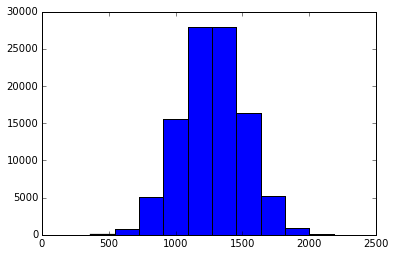
The central limit theorem suggests the sum of independent random variables would trend towards a normal distribution, not a uniformly random distribution, and indeed this is the case. This would be a very bad distribution for merging entropy. Under a uniform distribution picking any number was equally likely; now picking the midpoint seems like a good bet :)

On the flip side, perhaps you actually wanted to draw numbers from a normal distribution. In this case we’re not doing too bad, and can use this as a technique to create approximate normal distributions. However there are methods which seek instead to transform the input space that will be more efficient as they require fewer potentially costly random samples.

Breaking the Central Limit Theorem

Let’s look at all possible values that we can express by summing 3 integer values \(i, j, k \in [0, 1, 2, 3, 4]\). Let’s represent the summed values as colored circles:

For example, when \(i=0, j=1, k=2\) the sum will be \(i+j+k=3\) , and at the extent when \(i=4, j=4, k=4\) the sum is \(i+j+k=12\) .

The following psuedocode will add the sum of all three values to a row vector, a decomposition which may seem arbitrary at this point but will prove useful for visualization:

for i in range(5):
  for j in range(5):
    # Visualize the whole row of the inner loop. There will be 5^2 rows total.
    row = []
    for k in range(5):
      row.append(i + j + k)

All \(5^2\) inner loop rows are depicted below:

What if we stack the results? The Irwin-Hall distribution appears in the flesh!

Notice the stair-casing pattern. What if we could fold the values back on themselves to fill the empty space? Intuitively it will make a rectangle, when normalized this would be a uniform distribution. Let’s do exactly that: break this distribution with a modulo operator. In this case we are have \(x \mod 5\). We get a uniform distribution again!

While the order we looped over the elements is useful for visualization, it is not necessary for these results to hold; if the distribution is uniform, then we will be summing over the same values but with a random shuffling.

Combining Entropy Sources

With our newly found power to break the central limit theorem, what does the distribution of summed values look like? In this case, we plot the distribution of values modulo 255, the maximum value for one loop row:

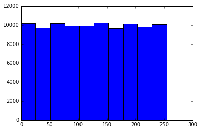
However, this may not be ideal for merging randomness in a more general case. If summed values are less than 255 (which is only true in the limit), the distribution will be Irwin-Hall again.

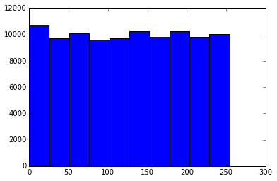
What are we to do? Luckily for us, there is a simple standard for this. Instead of summing the inputs together, we apply bitwise XOR. The distribution is also uniform for random inputs:

The ipython notebook for this can be found here.